Tutorial 7: Simulating Qiskit Metal design objects with palace using SQDMetal#
In this tutorial, we will cover how to do electrostatic and eigenmode simulations of a qubit-cavity system using palace.
Requirements:
☐ Ensure that SQDMetal is installed in your environment.
☐ Ensure that palace is installed in your environment. Instructions here.
[1]:
%load_ext autoreload
%autoreload 2
%matplotlib inline
[2]:
import os

os.environ["KMP_DUPLICATE_LIB_OK"]="TRUE"
os.environ["PMIX_MCA_gds"]="hash"

import gmsh

gmsh.initialize()

os.makedirs('sims', exist_ok=True)
Define the path to the palace executable
[3]:
path_to_palace = '/Users/shanto/LFL/palace/build/bin/palace'
Electrostatic Simulation#
We will be learning how to extract the capacitance matrix from an electrostatic simulation.
For a qubit-claw system#
Importing the relevant modules
[4]:
import pandas as pd
from qiskit_metal import Dict, MetalGUI, designs
from qiskit_metal.qlibrary.qubits.transmon_cross import TransmonCross
from qiskit_metal.qlibrary.terminations.launchpad_wb import LaunchpadWirebond
from qiskit_metal.qlibrary.terminations.open_to_ground import OpenToGround
from qiskit_metal.qlibrary.tlines.meandered import RouteMeander
from qiskit_metal.qlibrary.tlines.pathfinder import RoutePathfinder
We want to get the cap matrix for a system with TransmonCross, claw and ground (similar to the simulations we ran to build SQuADDS_DB)
[5]:
from squadds import Analyzer, SQuADDS_DB
FutureWarning: Module 'pyaedt' has become an alias to the new package structure. Please update you imports to use the new architecture based on 'ansys.aedt.core'. In addition, some files have been renamed to follow the PEP 8 naming convention. The old structure and file names will be deprecated in future versions, see https://aedt.docs.pyansys.com/version/stable/release_1_0.html
[6]:
# First, get a design from SQuADDS
db = SQuADDS_DB()
db.select_system("qubit")
db.select_qubit("TransmonCross")
df = db.create_system_df()
analyzer = Analyzer(db)

# Define target parameters for your qubit
target_params = {
    "qubit_frequency_GHz": 4.2,  # Example value
    "anharmonicity_MHz": -200    # Example value
}

# Find the closest design
results = analyzer.find_closest(target_params, num_top=1)
best_device = results.iloc[0]

# Get the design options
qubit_options = best_device["design_options"]
[7]:
# Set up chip design as planar
design = designs.DesignPlanar({}, overwrite_enabled=True)
# Create GUI
gui = MetalGUI(design)
# Qubit and a claw
# Create the TransmonCross object with the modified options
# Update only the position parameters
qubit_options["pos_x"] = '0.6075mm'
qubit_options["pos_y"] = '-1.464'
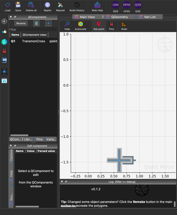
Q1 = TransmonCross(design, 'Q1', options=qubit_options)
gui.rebuild()
design.rebuild()
gui.autoscale()
gui.screenshot('sims/qubit.png')
02:50PM 05s CRITICAL [_qt_message_handler]: line: 0, func: None(), file: None  WARNING: Populating font family aliases took 284 ms. Replace uses of missing font family "Courier" with one that exists to avoid this cost.

02:50PM 05s CRITICAL [_qt_message_handler]: line: 0, func: None(), file: None  CRITICAL: <QNSWindow: 0x7f971d018da0; contentView=<QNSView: 0x7f971d018600; QCocoaWindow(0x7f971d0184f0, window=QWidgetWindow(0x7f971d017f90, name="MainWindowPlotWindow"))>> has active key-value observers (KVO)! These will stop working now that the window is recreated, and will result in exceptions when the observers are removed. Break in QCocoaWindow::recreateWindowIfNeeded to debug.

02:50PM 05s CRITICAL [_qt_message_handler]: line: 0, func: None(), file: None  CRITICAL: <QNSWindow: 0x7f971d022660; contentView=<QNSView: 0x7f971d021ec0; QCocoaWindow(0x7f971d021db0, window=QWidgetWindow(0x7f971d021830, name="ElementsWindowWindow"))>> has active key-value observers (KVO)! These will stop working now that the window is recreated, and will result in exceptions when the observers are removed. Break in QCocoaWindow::recreateWindowIfNeeded to debug.

02:50PM 05s CRITICAL [_qt_message_handler]: line: 0, func: None(), file: None  CRITICAL: <QNSWindow: 0x7f971d12a350; contentView=<QNSView: 0x7f971d129970; QCocoaWindow(0x7f971d129860, window=QWidgetWindow(0x7f971d129360, name="MainWindowWindow"))>> has active key-value observers (KVO)! These will stop working now that the window is recreated, and will result in exceptions when the observers are removed. Break in QCocoaWindow::recreateWindowIfNeeded to debug.

02:50PM 05s CRITICAL [_qt_message_handler]: line: 0, func: None(), file: None  CRITICAL: <QNSWindow: 0x7f971cfabb30; contentView=<QNSView: 0x7f971cfab390; QCocoaWindow(0x7f971cfab280, window=QWidgetWindow(0x7f971cfaad20, name="NetListWindowWindow"))>> has active key-value observers (KVO)! These will stop working now that the window is recreated, and will result in exceptions when the observers are removed. Break in QCocoaWindow::recreateWindowIfNeeded to debug.
Call the SQDMetal objects. Change the hyper-parameters as needed for a more accurate simulation.
[8]:
from SQDMetal.PALACE.Capacitance_Simulation import PALACE_Capacitance_Simulation

user_defined_options = {
                "mesh_refinement": 0,                             #refines mesh in PALACE - essetially divides every mesh element in half
                "dielectric_material": "silicon",                  #choose dielectric material - 'silicon' or 'sapphire'
                "solver_order": 1,                                 #increasing solver order increases accuracy of simulation, but significantly increases sim time
                "solver_tol": 1.0e-8,                              #error residual tolerance for iterative solver
                "solver_maxits": 500,                              #number of solver iterations
                "mesh_max": 120e-6,                                #maxiumum element size for the mesh in mm
                "mesh_sampling": 150,                              #number of points to mesh along a geometry
                "fillet_resolution":12,                            #number of vertices per quarter turn on a filleted path
                "num_cpus": 10,                                      #number of CPU cores to use for simulation
                "palace_dir":path_to_palace
                }
[9]:
#Creat the Palace Eigenmode simulation
cap_sim = PALACE_Capacitance_Simulation(name = 'transmon_cross_cap_sim',                                 #name of simulation
                                        metal_design = design,                                      #feed in qiskit metal design
                                        sim_parent_directory = "sims/",            #choose directory where mesh file, config file and HPC batch file will be saved
                                        mode = 'simPC',                                             #choose simulation mode 'HPC' or 'simPC'
                                        meshing = 'GMSH',                                           #choose meshing 'GMSH' or 'COMSOL'
                                        user_options = user_defined_options,                        #provide options chosen above
                                        view_design_gmsh_gui = False,                               #view design in GMSH gui
                                        create_files = True,
                                        )                                        #create mesh, config and HPC batch files

cap_sim.add_metallic(1, threshold=1e-10, fuse_threshold=1e-10)
cap_sim.add_ground_plane(threshold=1e-10)
To generate a fine mesh around our region of interest, we can use the fine_mesh_in_rectangle method by first getting the bounds of the region of interest.
[10]:
bounds = design.components["Q1"].qgeometry_bounds()
bounds
[10]:
array([ 0.3675, -1.704 , 0.9277, -1.224 ])
[11]:
#Fine-mesh the transmon cross qubit region
cap_sim.fine_mesh_in_rectangle(bounds[0]*1e-3, bounds[1]*1e-3, bounds[2]*1e-3, bounds[3]*1e-3, mesh_sampling=100, mesh_min=10e-3, mesh_max=125e-3)
[12]:
cap_sim.prepare_simulation()
You can check to see if all the metal components are correctly identified
[13]:
cap_sim.display_conductor_indices()
[13]:

Similarly, you can verify the mesh is correct by visualizing the mesh
[14]:
from SQDMetal.PALACE.Utilities.GMSH_Navigator import GMSH_Navigator

gmsh_nav = GMSH_Navigator(cap_sim.path_mesh)
gmsh_nav.open_GUI()
If all looks good, you can run the simulation
[15]:
cap_matrix =cap_sim.run()
>> /opt/homebrew/bin/mpirun -n 10 /Users/shanto/LFL/palace/build/bin/palace-arm64.bin transmon_cross_cap_sim.json

_____________     _______
_____   __   \____ __   /____ ____________
____   /_/  /  __ ` /  /  __ ` /  ___/  _ \
___   _____/  /_/  /  /  /_/  /  /__/  ___/
  /__/     \___,__/__/\___,__/\_____\_____/

Git changeset ID: v0.13.0-117-g748660c
Running with 10 MPI processes
Device configuration: cpu
Memory configuration: host-std
libCEED backend: /cpu/self/xsmm/blocked

Added 369 elements in 2 iterations of local bisection for under-resolved interior boundaries
Added 7772 duplicate vertices for interior boundaries in the mesh
Added 16409 duplicate boundary elements for interior boundaries in the mesh
Added 4040 boundary elements for material interfaces to the mesh
Finished partitioning mesh into 10 subdomains

Characteristic length and time scales:
 L₀ = 1.080e-02 m, t₀ = 3.602e-02 ns

Mesh curvature order: 1
Mesh bounding box:
 (Xmin, Ymin, Zmin) = (-5.400e-03, -3.600e-03, -7.500e-04) m
 (Xmax, Ymax, Zmax) = (+5.400e-03, +3.600e-03, +7.500e-04) m

Parallel Mesh Stats:

                minimum     average     maximum       total
 vertices          7422        7920        8388       79201
 edges            48320       49915       51242      499150
 faces            79214       80632       81980      806329
 elements         38316       38637       39385      386378
 neighbors            2           4           7

            minimum     maximum
 h      0.000552426   0.0217216
 kappa      1.01738     11.1252

Configuring Dirichlet BC at attributes:
 7, 1-3

Assembling system matrices, number of global unknowns:
 H1 (p = 1): 79201, ND (p = 1): 499150, RT (p = 1): 806329
 Operator assembly level: Partial
 Mesh geometries:
  Tetrahedron: P = 6, Q = 4 (quadrature order = 2)

Assembling multigrid hierarchy:
 Level 0 (p = 1): 79201 unknowns, 1105237 NNZ

Computing electrostatic fields for 3 terminal boundaries

It 1/3: Index = 1 (elapsed time = 4.20e-08 s)

  Residual norms for PCG solve
  0 KSP residual norm ||r||_B = 1.990521e+01
  1 KSP residual norm ||r||_B = 1.819635e+00
  2 KSP residual norm ||r||_B = 2.004853e-01
  3 KSP residual norm ||r||_B = 3.448215e-02
  4 KSP residual norm ||r||_B = 5.786581e-03
  5 KSP residual norm ||r||_B = 9.102787e-04
  6 KSP residual norm ||r||_B = 1.491365e-04
  7 KSP residual norm ||r||_B = 2.723162e-05
  8 KSP residual norm ||r||_B = 4.884593e-06
  9 KSP residual norm ||r||_B = 8.463240e-07
PCG solver converged in 9 iterations (avg. reduction factor: 1.236e-01)
 Sol. ||V|| = 1.770460e+02 (||RHS|| = 1.249420e+02)
 Field energy E = 1.624e+00 J
 Updating solution error estimates
 Wrote fields to disk for terminal 1

It 2/3: Index = 2 (elapsed time = 1.94e+00 s)

  Residual norms for PCG solve
  0 KSP residual norm ||r||_B = 8.173841e-01
  1 KSP residual norm ||r||_B = 8.983963e-02
  2 KSP residual norm ||r||_B = 1.454760e-02
  3 KSP residual norm ||r||_B = 2.128182e-03
  4 KSP residual norm ||r||_B = 3.333766e-04
  5 KSP residual norm ||r||_B = 6.577703e-05
  6 KSP residual norm ||r||_B = 1.180018e-05
  7 KSP residual norm ||r||_B = 1.987690e-06
  8 KSP residual norm ||r||_B = 3.601812e-07
  9 KSP residual norm ||r||_B = 6.149758e-08
PCG solver converged in 9 iterations (avg. reduction factor: 1.164e-01)
 Sol. ||V|| = 1.812398e+01 (||RHS|| = 1.571719e+01)
 Field energy E = 4.756e-02 J
 Updating solution error estimates
 Wrote fields to disk for terminal 2

It 3/3: Index = 3 (elapsed time = 3.66e+00 s)

  Residual norms for PCG solve
  0 KSP residual norm ||r||_B = 1.826447e+00
  1 KSP residual norm ||r||_B = 2.466585e-01
  2 KSP residual norm ||r||_B = 4.728945e-02
  3 KSP residual norm ||r||_B = 7.134869e-03
  4 KSP residual norm ||r||_B = 1.244552e-03
  5 KSP residual norm ||r||_B = 2.185094e-04
  6 KSP residual norm ||r||_B = 3.939749e-05
  7 KSP residual norm ||r||_B = 7.145503e-06
  8 KSP residual norm ||r||_B = 1.180785e-06
  9 KSP residual norm ||r||_B = 2.068803e-07
PCG solver converged in 9 iterations (avg. reduction factor: 1.260e-01)
 Sol. ||V|| = 3.791320e+01 (||RHS|| = 2.584766e+01)
 Field energy E = 2.559e-02 J
 Updating solution error estimates
 Wrote fields to disk for terminal 3

Completed 0 iterations of adaptive mesh refinement (AMR):
 Indicator norm = 5.098e-01, global unknowns = 79201
 Max. iterations = 0, tol. = 1.000e-02

Elapsed Time Report (s)           Min.        Max.        Avg.
==============================================================
Initialization                   8.096       8.106       8.101
Operator Construction            0.401       0.419       0.411
Linear Solve                     0.130       0.153       0.139
  Setup                          0.020       0.027       0.021
  Preconditioner                 0.498       0.532       0.519
Estimation                       0.072       0.093       0.083
  Construction                   5.676       5.676       5.676
  Solve                          1.764       1.773       1.766
Postprocessing                   0.371       0.393       0.380
Disk IO                          4.590       4.615       4.601
--------------------------------------------------------------
Total                           21.794      21.803      21.800

Error in plotting: 'Data array (V) not present in this dataset.'
[16]:
cdf = pd.DataFrame(cap_matrix)

# get rid of the first column
cdf = cdf.iloc[:, 1:]

# assigning the columns and indices based on our geometry
cdf.columns = ["ground", "claw", "cross"]
cdf.index = ["ground", "claw", "cross"]
cdf
[16]:
| ground | claw | cross | |
|---|---|---|---|
| ground | 8.621504e-12 | -2.458660e-13 | -1.239444e-13 |
| claw | -2.458660e-13 | 2.524815e-13 | -4.830456e-15 |
| cross | -1.239444e-13 | -4.830456e-15 | 1.358696e-13 |
The above dataframe is the capacitance matrix for our system in Farads.
To get a more accurate result - consider a higher order solver and a finer mesh.
Eigenmodal Simulation#
For a qubit-cavity system#
[17]:
# Import useful packages
import numpy as np
from qiskit_metal import MetalGUI, designs

from squadds.components.qubits import TransmonCross
For this example lets use an example geometry from Tutorial 5 and build the design with SQDMetal
[18]:
db.unselect_all()
db.select_system(["cavity_claw", "qubit"])
db.select_qubit("TransmonCross")
db.select_cavity_claw("RouteMeander")
db.select_resonator_type("quarter")
df = db.create_system_df()

analyzer.reload_db()
[19]:
target_params = {
                "qubit_frequency_GHz": 3.7,
                "resonator_type":"quarter",
                "anharmonicity_MHz": -210,
                "g_MHz": 100 # should provide a big punchout shift
                }

# computing the cavity frequency desired as per the design requirements
target_params["cavity_frequency_GHz"] = 2*(target_params["qubit_frequency_GHz"]+target_params["anharmonicity_MHz"]/1000)

results = analyzer.find_closest(target_params=target_params,num_top=1,metric="Euclidean")
results
Time taken to add the coupled H params: 4.424401044845581 seconds
[19]:
| index_qc | PI_qubit | date_created_qubit | group_qubit | institution_qubit | uploader_qubit | design_options_qubit | design_tool_qubit | claw_to_claw | claw_to_ground | ... | units_cavity_claw | renderer_options_cavity_claw | setup_cavity_claw | simulator_cavity_claw | design_options | EC | EJ | qubit_frequency_GHz | anharmonicity_MHz | g_MHz | |
|---|---|---|---|---|---|---|---|---|---|---|---|---|---|---|---|---|---|---|---|---|---|
| 12514 | 1900 | Eli Levenson-Falk, PhD | 2023-09-20-142549 | LFL | USC | Andre Kuo | {'aedt_hfss_capacitance': 0, 'aedt_hfss_induct... | qiskit-metal | 102.50358 | 94.66779 | ... | Hz | None | {'basis_order': 1, 'max_delta_f': 0.05, 'max_p... | Ansys HFSS | {'cavity_claw_options': {'coupler_type': 'CLT'... | 0.180488 | 10.278024 | 3.66213 | -205.109839 | 98.903433 |
1 rows × 41 columns
[20]:
data_qubit = analyzer.get_qubit_options(results)
data_cpw = analyzer.get_cpw_options(results)
data_coupler = analyzer.get_coupler_options(results)
LJs = analyzer.get_Ljs(results) # in nH
Creating a new design and gui object since we are running this in the same notebook.
[ ]:
# First delete components
design.delete_all_components()

# Close the GUI
gui.main_window.close()

# Forced garbage collection
gui = None
design = None
[23]:
design = designs.DesignPlanar({}, overwrite_enabled=True)
gui = MetalGUI(design)


# Set up chip dimensions
design.chips.main.size.size_x = '4.6mm'
design.chips.main.size.size_y = '2.4mm'
design.chips.main.size.size_z = '-280um'
design.chips.main.size.center_x = '0mm'
design.chips.main.size.center_y = '-1mm'
02:51PM 19s CRITICAL [_qt_message_handler]: line: 0, func: None(), file: None  CRITICAL: <QNSWindow: 0x7f97382d8840; contentView=<QNSView: 0x7f971d1b05a0; QCocoaWindow(0x7f971e2c8c30, window=QWidgetWindow(0x7f97381cdac0, name="MainWindowPlotWindow"))>> has active key-value observers (KVO)! These will stop working now that the window is recreated, and will result in exceptions when the observers are removed. Break in QCocoaWindow::recreateWindowIfNeeded to debug.

02:51PM 19s CRITICAL [_qt_message_handler]: line: 0, func: None(), file: None  CRITICAL: <QNSWindow: 0x7f9719fed4b0; contentView=<QNSView: 0x7f9719fecf40; QCocoaWindow(0x7f9719fece90, window=QWidgetWindow(0x7f972d533470, name="ElementsWindowWindow"))>> has active key-value observers (KVO)! These will stop working now that the window is recreated, and will result in exceptions when the observers are removed. Break in QCocoaWindow::recreateWindowIfNeeded to debug.

02:51PM 19s CRITICAL [_qt_message_handler]: line: 0, func: None(), file: None  CRITICAL: <QNSWindow: 0x7f972b3eadd0; contentView=<QNSView: 0x7f972b3ea650; QCocoaWindow(0x7f972b3ea540, window=QWidgetWindow(0x7f972b3ea040, name="MainWindowWindow"))>> has active key-value observers (KVO)! These will stop working now that the window is recreated, and will result in exceptions when the observers are removed. Break in QCocoaWindow::recreateWindowIfNeeded to debug.

02:51PM 19s CRITICAL [_qt_message_handler]: line: 0, func: None(), file: None  CRITICAL: <QNSWindow: 0x7f9719ff4b00; contentView=<QNSView: 0x7f9719ff4590; QCocoaWindow(0x7f9719ff44e0, window=QWidgetWindow(0x7f972d53b930, name="NetListWindowWindow"))>> has active key-value observers (KVO)! These will stop working now that the window is recreated, and will result in exceptions when the observers are removed. Break in QCocoaWindow::recreateWindowIfNeeded to debug.
Lets create the qubit with a junction and a claw
Qubit (with a junction) and Claw#
[24]:
from SQDMetal.Comps.Capacitors import CapacitorProngPin
from SQDMetal.Comps.Junctions import JunctionDolanPinStretch
from SQDMetal.Comps.Xmon import Xmon
[25]:
# Calculate vBar_gap and hBar_gap
def extract_um(value: str) -> float:
    """Extract float from '30um'."""
    return float(value.replace('um', ''))

# Unpack parameters from data_qubit
cross_width = extract_um(data_qubit['cross_width'][0])
cross_length = extract_um(data_qubit['cross_length'][0])
cross_gap = extract_um(data_qubit['cross_gap'][0])

# Now create the Xmon
xmon = Xmon(
    design,
    'xmon',
    options=Dict(
        pos_x = '0.375mm',
        pos_y = '-1.3',
        hBar_width = f"{cross_width}um",
        vBar_width = f"{cross_width}um",
        vBar_gap = f"{cross_gap}um",
        hBar_gap = f"{cross_gap}um",
        cross_width = f"{2*cross_length}um",
        cross_height = f"{2*cross_length}um",
        gap_up = data_qubit['cross_gap'][0],
        gap_left = data_qubit['cross_gap'][0],
        gap_right = data_qubit['cross_gap'][0],
        gap_down = data_qubit['cross_gap'][0]
    )
)
[26]:
# Claw
prong_length = extract_um(data_qubit['claw_length'][0]) - extract_um(data_qubit['claw_width'][0])
pin_gap_side = extract_um(data_qubit['claw_gap'][0])+extract_um(data_qubit['cross_gap'][0])+extract_um(data_qubit['ground_spacing'][0])

claw = CapacitorProngPin(
    design,
    'claw',
    options=Dict(
        pin_inputs=Dict(start_pin=Dict(component='xmon', pin='up')),
        prong_width = data_qubit['claw_width'][0],
        pad_thickness = data_qubit['claw_width'][0],
        gap_front = data_qubit['cross_gap'][0],
        gap_back = data_qubit['claw_gap'][0],
        gap_side = data_qubit['claw_gap'][0],
        prong_length = f"{prong_length}um",
        pin_gap_side = f"{pin_gap_side}um"
    )
)
[27]:
# Junction
junction = JunctionDolanPinStretch(design, 'junction', options=Dict(pin_inputs=Dict(start_pin=Dict(component='xmon',pin='right')),
                                                         dist_extend=data_qubit['cross_gap'][0],
                                                         layer=2,
                                                         finger_width='0.4um', t_pad_size='0.385um',
                                                         squid_width='5.4um', prong_width='0.9um'))
Resonator and Feedline#
Now lets add the resonator and feedline
[28]:
# Lauchpad 1
x1 = '-2mm'
y1 = '0mm'
launch_options1 = dict(chip='main', pos_x=x1, pos_y=y1, orientation='360', lead_length='30um', pad_height='103um',
                      pad_width='103um', pad_gap='60um', trace_width = data_cpw["trace_width"], trace_gap = data_cpw["trace_gap"])
LP1 = LaunchpadWirebond(design, 'LP1', options = launch_options1)

# Launchpad 2
x2 = '2mm'
y1 = '0mm'
launch_options2 = dict(chip='main', pos_x=x2, pos_y=y1, orientation='180', lead_length='30um', pad_height='103um',
                      pad_width='103um', pad_gap='60um', trace_width = data_cpw["trace_width"], trace_gap = data_cpw["trace_gap"])
LP2 = LaunchpadWirebond(design, 'LP2', options = launch_options2)

# Using path finder to connect the two launchpads
feedline = RoutePathfinder(design, 'feedline', options = dict(chip='main', trace_width = data_cpw["trace_width"],
                                            trace_gap = data_cpw["trace_gap"],
                                            fillet='90um',
                                            hfss_wire_bonds = True,
                                            lead=dict(end_straight='0.1mm'),
                                            pin_inputs=Dict(
                                                start_pin=Dict(
                                                    component='LP1',
                                                    pin='tie'),
                                                end_pin=Dict(
                                                    component='LP2',
                                                    pin='tie')
                                            )))
[29]:
#open to ground for resonator
otg1 = OpenToGround(design, 'otg1', options=dict(chip='main', pos_x='-0.2mm',  pos_y='-40um', orientation = 180))


# Resonator and feedline gap width (W) and center conductor width (S)
design.variables['cpw_width'] = data_cpw["trace_width"]
design.variables['cpw_gap'] = data_cpw["trace_gap"]

# Use RouteMeander to fix the total length of the resonator
res1 = RouteMeander(design, 'resonator',  Dict(
        trace_width ='10um',
        trace_gap ='6um',
        total_length='3.7mm',
        hfss_wire_bonds = False,
        fillet='99.9 um',
        lead = dict(start_straight='300um'),
        pin_inputs=Dict(
        start_pin=Dict(component= 'otg1', pin= 'open'),
        end_pin=Dict(component= 'claw', pin= 'a')), ))
Check the design
[30]:
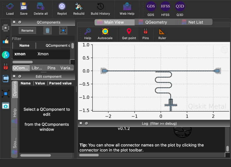
# rebuild the GUI
design.rebuild()
gui.rebuild()
gui.autoscale()
gui.screenshot('sims/qubit-cavity.png')
Define the hyper-parameters for the eigenmode simulation
[31]:
from SQDMetal.PALACE.Eigenmode_Simulation import PALACE_Eigenmode_Simulation

#Eigenmode Simulation Options
user_defined_options = {
                 "mesh_refinement":  0,                             #refines mesh in PALACE - essetially divides every mesh element in half
                 "dielectric_material": "silicon",                  #choose dielectric material - 'silicon' or 'sapphire'
                 "starting_freq": 2e9,                              #starting frequency in Hz
                 "number_of_freqs": 6,                              #number of eigenmodes to find
                 "solns_to_save": 6,                                #number of electromagnetic field visualizations to save
                 "solver_order": 1,                                 #increasing solver order increases accuracy of simulation, but significantly increases sim time
                 "solver_tol": 1.0e-3,                              #error residual tolerance foriterative solver
                 "solver_maxits": 3,                              #number of solver iterations
                 "mesh_max": 120e-3,                                #maxiumum element size for the mesh in mm
                 "mesh_min": 10e-3,                                 #minimum element size for the mesh in mm
                 "mesh_sampling": 130,                              #number of points to mesh along a geometry
                 "fillet_resolution":12,
                 "num_cpus": 10,                                      #number of CPU cores to use for simulation
                 "palace_dir":path_to_palace
                }

#Creat the Palace Eigenmode simulation
eigen_sim = PALACE_Eigenmode_Simulation(name ='qubit-cavity-eig-test',                              #name of simulation
                                        metal_design = design,                                      #feed in qiskit metal design
                                        sim_parent_directory = "sims/",            #choose directory where mesh file, config file and HPC batch file will be saved
                                        mode = 'simPC',                                               #choose simulation mode 'HPC' or 'simPC'
                                        meshing = 'GMSH',                                         #choose meshing 'GMSH' or 'COMSOL'
                                        user_options = user_defined_options,                        #provide options chosen above
                                        view_design_gmsh_gui = False,                               #view design in GMSH gui
                                        create_files = True)                                        #create mesh, config and HPC batch files
Assigning the materials to the interfaces, add ports to the design, and add some mesh.
[32]:
from SQDMetal.Utilities.Materials import MaterialInterface

eigen_sim.add_metallic(1, threshold=1e-10, fuse_threshold=1e-10)
eigen_sim.add_ground_plane(threshold=1e-10)

#Fine-mesh the transmon cross qubit region
eigen_sim.fine_mesh_in_rectangle(0.2875e-3, -1.2e-3, 0.63e-3, -1.72e-3, min_size=15e-6, max_size=120e-6)

#Add in the RF ports
eigen_sim.create_port_CPW_on_Launcher('LP1', 20e-6)
eigen_sim.create_port_CPW_on_Launcher('LP2', 20e-6)
eigen_sim.create_port_JosephsonJunction('junction', L_J=LJs[0]*1e-9, C_J=10e-15) # Guessing the C_J value really

# #Fine-mesh routed paths
eigen_sim.fine_mesh_around_comp_boundaries(['feedline', 'resonator'], min_size=25e-6, max_size=250e-6)
eigen_sim.fine_mesh_around_comp_boundaries(['xmon'], min_size=14e-6, max_size=75e-6)

eigen_sim.setup_EPR_interfaces(metal_air=MaterialInterface('Aluminium-Vacuum'), substrate_air=MaterialInterface('Silicon-Vacuum'), substrate_metal=MaterialInterface('Silicon-Aluminium'))
[33]:
eigen_sim.prepare_simulation()
Checking the meshfile
[ ]:
gmsh_nav = GMSH_Navigator(eigen_sim.path_mesh)
gmsh_nav.open_GUI()
If all looks good, lets run the simulation
NOTE: If you are using a palace build that is from 2025, you will need to remove the Excitation key from the LumpedPort boundary condition in the sim_config.json file so please execute the following cell.
If you are using a palace build that is from 2024 or older, you should skip this cell.
[ ]:
import json

with open(eigen_sim._sim_config) as file:
    sim_config_dict = json.load(file)

del sim_config_dict["Boundaries"]["LumpedPort"][0]["Excitation"]

with open(eigen_sim._sim_config, 'w') as file:
    json.dump(sim_config_dict, file, indent=4)
[34]:
eigen_sim.run()
>> /opt/homebrew/bin/mpirun -n 10 /Users/shanto/LFL/palace/build/bin/palace-arm64.bin qubit-cavity-eig-test.json
_____________ _______
_____ __ \____ __ /____ ____________
____ /_/ / __ ` / / __ ` / ___/ _ \
___ _____/ /_/ / / /_/ / /__/ ___/
/__/ \___,__/__/\___,__/\_____\_____/
Git changeset ID: v0.13.0-117-g748660c
Running with 10 MPI processes
Device configuration: cpu
Memory configuration: host-std
libCEED backend: /cpu/self/xsmm/blocked
Added 2574 elements in 2 iterations of local bisection for under-resolved interior boundaries
Added 5333 duplicate vertices for interior boundaries in the mesh
Added 12701 duplicate boundary elements for interior boundaries in the mesh
Added 1550 boundary elements for material interfaces to the mesh
Finished partitioning mesh into 10 subdomains
Characteristic length and time scales:
L₀ = 5.520e-03 m, t₀ = 1.841e-02 ns
Mesh curvature order: 1
Mesh bounding box:
(Xmin, Ymin, Zmin) = (-2.760e-03, -2.440e-03, -2.800e-04) m
(Xmax, Ymax, Zmax) = (+2.760e-03, +4.400e-04, +2.800e-04) m
Parallel Mesh Stats:
minimum average maximum total
vertices 2786 3522 3859 35223
edges 18749 20919 22124 209195
faces 31110 32653 33699 326538
elements 15011 15256 15457 152568
neighbors 2 4 5
minimum maximum
h 0.000513927 0.0271869
kappa 1.01967 157.435
Configuring Robin absorbing BC (order 1) at attributes:
13
Configuring Robin impedance BC for lumped ports at attributes:
5: Rs = 6.667e+01 Ω/sq, n = (+0.0, +0.0, +1.0)
6: Rs = 6.667e+01 Ω/sq, n = (+0.0, +0.0, -1.0)
7: Rs = 6.667e+01 Ω/sq, n = (-0.0, +0.0, +1.0)
8: Rs = 6.667e+01 Ω/sq, n = (+0.0, +0.0, -1.0)
9: Ls = 5.725e-09 H/sq, Cs = 2.778e-14 F/sq, n = (+0.0, +0.0, +1.0)
Configuring lumped port circuit properties:
Index = 1: R = 5.000e+01 Ω
Index = 2: R = 5.000e+01 Ω
Index = 3: L = 1.590e-08 H, C = 1.000e-14 F
Configuring lumped port excitation source term at attributes:
5: Index = 1
6: Index = 1
Configuring Dirichlet PEC BC at attributes:
1-4
Assembling system matrices, number of global unknowns:
H1 (p = 1): 35223, ND (p = 1): 209195, RT (p = 1): 326538
Operator assembly level: Partial
Mesh geometries:
Tetrahedron: P = 6, Q = 4 (quadrature order = 2)
Configuring SLEPc eigenvalue solver:
Scaling γ = 4.711e+02, δ = 1.089e-05
Configuring divergence-free projection
Using random starting vector
Shift-and-invert σ = 2.000e+00 GHz (2.314e-01)
Assembling multigrid hierarchy:
Level 0 (p = 1): 209195 unknowns, 3111237 NNZ
Level 0 (auxiliary) (p = 1): 35223 unknowns, 467972 NNZ
#PETSc Option Table entries:
-eps_monitor # (source: code)
#End of PETSc Option Table entries
Residual norms for FGMRES solve
0 (restart 0) KSP residual norm 1.430279e+03
1 (restart 0) KSP residual norm 1.025289e-01
FGMRES solver converged in 1 iteration (avg. reduction factor: 7.168e-05)
Residual norms for FGMRES solve
0 (restart 0) KSP residual norm 3.363427e+02
1 (restart 0) KSP residual norm 4.284830e-01
2 (restart 0) KSP residual norm 5.323492e-02
FGMRES solver converged in 2 iterations (avg. reduction factor: 1.258e-02)
Residual norms for FGMRES solve
0 (restart 0) KSP residual norm 4.995177e+01
1 (restart 0) KSP residual norm 2.962309e-01
2 (restart 0) KSP residual norm 1.384106e-01
3 (restart 0) KSP residual norm 4.256018e-03
FGMRES solver converged in 3 iterations (avg. reduction factor: 4.400e-02)
Residual norms for FGMRES solve
0 (restart 0) KSP residual norm 2.399569e+02
1 (restart 0) KSP residual norm 1.230768e+00
2 (restart 0) KSP residual norm 5.933160e-01
3 (restart 0) KSP residual norm 2.217576e-02
FGMRES solver converged in 3 iterations (avg. reduction factor: 4.521e-02)
Residual norms for FGMRES solve
0 (restart 0) KSP residual norm 1.244339e+02
1 (restart 0) KSP residual norm 1.137913e+00
2 (restart 0) KSP residual norm 3.299754e-01
3 (restart 0) KSP residual norm 1.271091e-02
FGMRES solver converged in 3 iterations (avg. reduction factor: 4.675e-02)
Residual norms for FGMRES solve
0 (restart 0) KSP residual norm 2.330694e+02
1 (restart 0) KSP residual norm 6.423500e+00
2 (restart 0) KSP residual norm 2.903788e+00
3 (restart 0) KSP residual norm 5.072627e-02
FGMRES solver converged in 3 iterations (avg. reduction factor: 6.015e-02)
Residual norms for FGMRES solve
0 (restart 0) KSP residual norm 1.177260e+02
1 (restart 0) KSP residual norm 1.965855e+01
2 (restart 0) KSP residual norm 1.019226e+01
3 (restart 0) KSP residual norm 4.281215e-02
FGMRES solver converged in 3 iterations (avg. reduction factor: 7.138e-02)
Residual norms for FGMRES solve
0 (restart 0) KSP residual norm 7.166516e+01
1 (restart 0) KSP residual norm 1.882151e+01
2 (restart 0) KSP residual norm 8.034346e+00
3 (restart 1) KSP residual norm 8.581616e-02
FGMRES solver did NOT converge in 3 iterations (avg. reduction factor: 1.062e-01)
--> Warning!
Linear solver did not converge, norm(Ax-b)/norm(b) = 1.197e-03 (norm(b) = 7.167e+01)!
Residual norms for FGMRES solve
0 (restart 0) KSP residual norm 4.438828e+01
1 (restart 0) KSP residual norm 3.915629e+01
2 (restart 0) KSP residual norm 2.771825e+01
3 (restart 1) KSP residual norm 1.376060e-01
FGMRES solver did NOT converge in 3 iterations (avg. reduction factor: 1.458e-01)
--> Warning!
Linear solver did not converge, norm(Ax-b)/norm(b) = 3.100e-03 (norm(b) = 4.439e+01)!
Residual norms for FGMRES solve
0 (restart 0) KSP residual norm 1.881353e+01
1 (restart 0) KSP residual norm 1.794439e+01
2 (restart 0) KSP residual norm 1.621458e+01
3 (restart 1) KSP residual norm 2.216238e-01
FGMRES solver did NOT converge in 3 iterations (avg. reduction factor: 2.275e-01)
--> Warning!
Linear solver did not converge, norm(Ax-b)/norm(b) = 1.178e-02 (norm(b) = 1.881e+01)!
Residual norms for FGMRES solve
0 (restart 0) KSP residual norm 7.437849e+01
1 (restart 0) KSP residual norm 4.763870e+01
2 (restart 0) KSP residual norm 2.423142e+01
3 (restart 1) KSP residual norm 1.437091e-01
FGMRES solver did NOT converge in 3 iterations (avg. reduction factor: 1.246e-01)
--> Warning!
Linear solver did not converge, norm(Ax-b)/norm(b) = 1.932e-03 (norm(b) = 7.438e+01)!
Residual norms for FGMRES solve
0 (restart 0) KSP residual norm 3.741477e+01
1 (restart 0) KSP residual norm 1.922261e+01
2 (restart 0) KSP residual norm 1.103699e+01
3 (restart 1) KSP residual norm 1.051296e-01
FGMRES solver did NOT converge in 3 iterations (avg. reduction factor: 1.411e-01)
--> Warning!
Linear solver did not converge, norm(Ax-b)/norm(b) = 2.810e-03 (norm(b) = 3.741e+01)!
Residual norms for FGMRES solve
0 (restart 0) KSP residual norm 5.816988e+01
1 (restart 0) KSP residual norm 1.515933e+01
2 (restart 0) KSP residual norm 4.254473e+00
3 (restart 1) KSP residual norm 1.630771e-01
FGMRES solver did NOT converge in 3 iterations (avg. reduction factor: 1.410e-01)
--> Warning!
Linear solver did not converge, norm(Ax-b)/norm(b) = 2.803e-03 (norm(b) = 5.817e+01)!
Residual norms for FGMRES solve
0 (restart 0) KSP residual norm 9.802764e+01
1 (restart 0) KSP residual norm 1.492573e+01
2 (restart 0) KSP residual norm 3.576847e+00
3 (restart 1) KSP residual norm 2.360518e-01
FGMRES solver did NOT converge in 3 iterations (avg. reduction factor: 1.340e-01)
--> Warning!
Linear solver did not converge, norm(Ax-b)/norm(b) = 2.408e-03 (norm(b) = 9.803e+01)!
Residual norms for FGMRES solve
0 (restart 0) KSP residual norm 7.515375e+01
1 (restart 0) KSP residual norm 2.017880e+01
2 (restart 0) KSP residual norm 1.033416e+01
3 (restart 1) KSP residual norm 2.479146e-01
FGMRES solver did NOT converge in 3 iterations (avg. reduction factor: 1.489e-01)
--> Warning!
Linear solver did not converge, norm(Ax-b)/norm(b) = 3.299e-03 (norm(b) = 7.515e+01)!
Residual norms for FGMRES solve
0 (restart 0) KSP residual norm 2.893357e+01
1 (restart 0) KSP residual norm 1.684603e+01
2 (restart 0) KSP residual norm 6.739747e+00
3 (restart 1) KSP residual norm 3.242989e-01
FGMRES solver did NOT converge in 3 iterations (avg. reduction factor: 2.238e-01)
--> Warning!
Linear solver did not converge, norm(Ax-b)/norm(b) = 1.121e-02 (norm(b) = 2.893e+01)!
Residual norms for FGMRES solve
0 (restart 0) KSP residual norm 6.275288e+01
1 (restart 0) KSP residual norm 3.481004e+01
2 (restart 0) KSP residual norm 8.956162e+00
3 (restart 1) KSP residual norm 2.241883e-01
FGMRES solver did NOT converge in 3 iterations (avg. reduction factor: 1.529e-01)
--> Warning!
Linear solver did not converge, norm(Ax-b)/norm(b) = 3.573e-03 (norm(b) = 6.275e+01)!
Residual norms for FGMRES solve
0 (restart 0) KSP residual norm 9.813501e+01
1 (restart 0) KSP residual norm 5.771674e+01
2 (restart 0) KSP residual norm 2.303109e+01
3 (restart 1) KSP residual norm 3.287289e-01
FGMRES solver did NOT converge in 3 iterations (avg. reduction factor: 1.496e-01)
--> Warning!
Linear solver did not converge, norm(Ax-b)/norm(b) = 3.350e-03 (norm(b) = 9.814e+01)!
Residual norms for FGMRES solve
0 (restart 0) KSP residual norm 7.720080e+01
1 (restart 0) KSP residual norm 6.971510e+01
2 (restart 0) KSP residual norm 5.686810e+01
3 (restart 1) KSP residual norm 6.714601e-01
FGMRES solver did NOT converge in 3 iterations (avg. reduction factor: 2.057e-01)
--> Warning!
Linear solver did not converge, norm(Ax-b)/norm(b) = 8.698e-03 (norm(b) = 7.720e+01)!
Residual norms for FGMRES solve
0 (restart 0) KSP residual norm 7.638992e+01
1 (restart 0) KSP residual norm 5.367765e+01
2 (restart 0) KSP residual norm 3.439303e+01
3 (restart 1) KSP residual norm 4.234628e-01
FGMRES solver did NOT converge in 3 iterations (avg. reduction factor: 1.770e-01)
--> Warning!
Linear solver did not converge, norm(Ax-b)/norm(b) = 5.543e-03 (norm(b) = 7.639e+01)!
Residual norms for FGMRES solve
0 (restart 0) KSP residual norm 4.046472e+01
1 (restart 0) KSP residual norm 3.724911e+01
2 (restart 0) KSP residual norm 2.931985e+01
3 (restart 1) KSP residual norm 5.039609e-01
FGMRES solver did NOT converge in 3 iterations (avg. reduction factor: 2.318e-01)
--> Warning!
Linear solver did not converge, norm(Ax-b)/norm(b) = 1.245e-02 (norm(b) = 4.046e+01)!
Eigenvalue approximations and residual norms for solve.
1 EPS nconv=3 first unconverged value (error) -5.99788e-05+0.00236959i (7.88472977e-03)
Residual norms for FGMRES solve
0 (restart 0) KSP residual norm 9.338336e+01
1 (restart 0) KSP residual norm 6.841398e+01
2 (restart 0) KSP residual norm 1.550734e+01
3 (restart 1) KSP residual norm 3.357722e-01
FGMRES solver did NOT converge in 3 iterations (avg. reduction factor: 1.532e-01)
--> Warning!
Linear solver did not converge, norm(Ax-b)/norm(b) = 3.596e-03 (norm(b) = 9.338e+01)!
Residual norms for FGMRES solve
0 (restart 0) KSP residual norm 3.848724e+01
1 (restart 0) KSP residual norm 3.529266e+01
2 (restart 0) KSP residual norm 1.276312e+01
3 (restart 1) KSP residual norm 4.107400e-01
FGMRES solver did NOT converge in 3 iterations (avg. reduction factor: 2.202e-01)
--> Warning!
Linear solver did not converge, norm(Ax-b)/norm(b) = 1.067e-02 (norm(b) = 3.849e+01)!
Residual norms for FGMRES solve
0 (restart 0) KSP residual norm 2.146016e+01
1 (restart 0) KSP residual norm 1.793989e+01
2 (restart 0) KSP residual norm 3.548481e+00
3 (restart 1) KSP residual norm 3.491101e-01
FGMRES solver did NOT converge in 3 iterations (avg. reduction factor: 2.534e-01)
--> Warning!
Linear solver did not converge, norm(Ax-b)/norm(b) = 1.627e-02 (norm(b) = 2.146e+01)!
Residual norms for FGMRES solve
0 (restart 0) KSP residual norm 2.626228e+01
1 (restart 0) KSP residual norm 1.619951e+01
2 (restart 0) KSP residual norm 9.739910e+00
3 (restart 1) KSP residual norm 2.572633e-01
FGMRES solver did NOT converge in 3 iterations (avg. reduction factor: 2.140e-01)
--> Warning!
Linear solver did not converge, norm(Ax-b)/norm(b) = 9.796e-03 (norm(b) = 2.626e+01)!
Residual norms for FGMRES solve
0 (restart 0) KSP residual norm 6.053278e+01
1 (restart 0) KSP residual norm 3.773032e+01
2 (restart 0) KSP residual norm 9.383100e+00
3 (restart 1) KSP residual norm 3.134839e-01
FGMRES solver did NOT converge in 3 iterations (avg. reduction factor: 1.730e-01)
--> Warning!
Linear solver did not converge, norm(Ax-b)/norm(b) = 5.179e-03 (norm(b) = 6.053e+01)!
Residual norms for FGMRES solve
0 (restart 0) KSP residual norm 3.068695e+01
1 (restart 0) KSP residual norm 2.227342e+01
2 (restart 0) KSP residual norm 1.148230e+01
3 (restart 1) KSP residual norm 3.263643e-01
FGMRES solver did NOT converge in 3 iterations (avg. reduction factor: 2.199e-01)
--> Warning!
Linear solver did not converge, norm(Ax-b)/norm(b) = 1.064e-02 (norm(b) = 3.069e+01)!
Residual norms for FGMRES solve
0 (restart 0) KSP residual norm 3.999870e+01
1 (restart 0) KSP residual norm 3.774763e+01
2 (restart 0) KSP residual norm 3.236711e+01
3 (restart 1) KSP residual norm 4.540024e-01
FGMRES solver did NOT converge in 3 iterations (avg. reduction factor: 2.247e-01)
--> Warning!
Linear solver did not converge, norm(Ax-b)/norm(b) = 1.135e-02 (norm(b) = 4.000e+01)!
Residual norms for FGMRES solve
0 (restart 0) KSP residual norm 5.487457e+01
1 (restart 0) KSP residual norm 1.479069e+01
2 (restart 0) KSP residual norm 3.900170e+00
3 (restart 1) KSP residual norm 3.848939e-01
FGMRES solver did NOT converge in 3 iterations (avg. reduction factor: 1.914e-01)
--> Warning!
Linear solver did not converge, norm(Ax-b)/norm(b) = 7.014e-03 (norm(b) = 5.487e+01)!
Residual norms for FGMRES solve
0 (restart 0) KSP residual norm 2.998237e+01
1 (restart 0) KSP residual norm 2.593476e+01
2 (restart 0) KSP residual norm 1.755288e+01
3 (restart 1) KSP residual norm 2.091052e-01
FGMRES solver did NOT converge in 3 iterations (avg. reduction factor: 1.911e-01)
--> Warning!
Linear solver did not converge, norm(Ax-b)/norm(b) = 6.974e-03 (norm(b) = 2.998e+01)!
2 EPS nconv=3 first unconverged value (error) -6.48921e-06+0.00237218i (3.24934625e-03)
Residual norms for FGMRES solve
0 (restart 0) KSP residual norm 9.155483e+01
1 (restart 0) KSP residual norm 7.560587e+01
2 (restart 0) KSP residual norm 5.350513e+01
3 (restart 1) KSP residual norm 3.359118e-01
FGMRES solver did NOT converge in 3 iterations (avg. reduction factor: 1.542e-01)
--> Warning!
Linear solver did not converge, norm(Ax-b)/norm(b) = 3.669e-03 (norm(b) = 9.155e+01)!
Residual norms for FGMRES solve
0 (restart 0) KSP residual norm 4.328329e+01
1 (restart 0) KSP residual norm 5.176884e+00
2 (restart 0) KSP residual norm 2.643262e+00
3 (restart 1) KSP residual norm 7.311450e-02
FGMRES solver did NOT converge in 3 iterations (avg. reduction factor: 1.191e-01)
--> Warning!
Linear solver did not converge, norm(Ax-b)/norm(b) = 1.689e-03 (norm(b) = 4.328e+01)!
Residual norms for FGMRES solve
0 (restart 0) KSP residual norm 2.654228e+01
1 (restart 0) KSP residual norm 2.470876e+01
2 (restart 0) KSP residual norm 1.929156e+01
3 (restart 1) KSP residual norm 1.585680e-01
FGMRES solver did NOT converge in 3 iterations (avg. reduction factor: 1.815e-01)
--> Warning!
Linear solver did not converge, norm(Ax-b)/norm(b) = 5.974e-03 (norm(b) = 2.654e+01)!
Residual norms for FGMRES solve
0 (restart 0) KSP residual norm 2.883958e+01
1 (restart 0) KSP residual norm 2.513077e+01
2 (restart 0) KSP residual norm 1.667734e+01
3 (restart 1) KSP residual norm 1.766759e-01
FGMRES solver did NOT converge in 3 iterations (avg. reduction factor: 1.830e-01)
--> Warning!
Linear solver did not converge, norm(Ax-b)/norm(b) = 6.126e-03 (norm(b) = 2.884e+01)!
Residual norms for FGMRES solve
0 (restart 0) KSP residual norm 2.437399e+01
1 (restart 0) KSP residual norm 2.136668e+01
2 (restart 0) KSP residual norm 1.101456e+01
3 (restart 1) KSP residual norm 1.470401e-01
FGMRES solver did NOT converge in 3 iterations (avg. reduction factor: 1.820e-01)
--> Warning!
Linear solver did not converge, norm(Ax-b)/norm(b) = 6.033e-03 (norm(b) = 2.437e+01)!
Residual norms for FGMRES solve
0 (restart 0) KSP residual norm 2.322936e+01
1 (restart 0) KSP residual norm 1.508105e+01
2 (restart 0) KSP residual norm 2.701484e+00
3 (restart 1) KSP residual norm 1.939744e-01
FGMRES solver did NOT converge in 3 iterations (avg. reduction factor: 2.029e-01)
--> Warning!
Linear solver did not converge, norm(Ax-b)/norm(b) = 8.350e-03 (norm(b) = 2.323e+01)!
Residual norms for FGMRES solve
0 (restart 0) KSP residual norm 1.838854e+01
1 (restart 0) KSP residual norm 1.748158e+01
2 (restart 0) KSP residual norm 1.322922e+01
3 (restart 1) KSP residual norm 1.401764e-01
FGMRES solver did NOT converge in 3 iterations (avg. reduction factor: 1.968e-01)
--> Warning!
Linear solver did not converge, norm(Ax-b)/norm(b) = 7.623e-03 (norm(b) = 1.839e+01)!
Residual norms for FGMRES solve
0 (restart 0) KSP residual norm 3.768894e+01
1 (restart 0) KSP residual norm 2.925392e+01
2 (restart 0) KSP residual norm 1.883577e+01
3 (restart 1) KSP residual norm 3.743840e-01
FGMRES solver did NOT converge in 3 iterations (avg. reduction factor: 2.150e-01)
--> Warning!
Linear solver did not converge, norm(Ax-b)/norm(b) = 9.934e-03 (norm(b) = 3.769e+01)!
Residual norms for FGMRES solve
0 (restart 0) KSP residual norm 6.222283e+01
1 (restart 0) KSP residual norm 2.570920e+01
2 (restart 0) KSP residual norm 1.159447e+01
3 (restart 1) KSP residual norm 3.743351e-01
FGMRES solver did NOT converge in 3 iterations (avg. reduction factor: 1.819e-01)
--> Warning!
Linear solver did not converge, norm(Ax-b)/norm(b) = 6.016e-03 (norm(b) = 6.222e+01)!
3 EPS nconv=6 first unconverged value (error) -5.03846e-05+0.00284044i (5.04194851e-03)
Linear eigensolve converged (6 eigenpairs) due to CONVERGED_TOL; iterations 3
Total number of linear systems solved: 39
Total number of linear solver iterations: 114
Found 6 converged eigenvalues (first = -1.642e-05+3.629e-01i)
Computing solution error estimates and performing postprocessing
m Re{ω}/2π (GHz) Im{ω}/2π (GHz) Bkwd. Error Abs. Error
=============================================================================
1 +3.136773e+00 +1.419088e-04 +7.453931e-09 +1.332296e-03
Wrote mode 1 to disk
2 +7.182393e+00 +5.380575e-02 +1.006761e-06 +1.799511e-01
Wrote mode 2 to disk
3 +7.984742e+00 +6.056005e-02 +1.045471e-06 +1.868715e-01
Wrote mode 3 to disk
4 +9.637756e+00 +4.853371e-02 +1.024503e-06 +1.831260e-01
Wrote mode 4 to disk
5 +9.940094e+00 +7.946123e-02 +1.765758e-06 +3.156232e-01
Wrote mode 5 to disk
6 +1.069663e+01 +2.472286e-01 +8.803714e-07 +1.573643e-01
Wrote mode 6 to disk
Completed 0 iterations of adaptive mesh refinement (AMR):
Indicator norm = 4.003e-01, global unknowns = 209195
Max. iterations = 0, tol. = 1.000e-02
Elapsed Time Report (s) Min. Max. Avg.
==============================================================
Initialization 3.397 3.417 3.405
Operator Construction 3.128 3.143 3.137
Linear Solve 5.972 6.088 6.019
Setup 0.077 0.079 0.078
Preconditioner 17.736 17.795 17.768
Eigenvalue Solve 3.406 3.462 3.437
Div.-Free Projection 13.755 13.848 13.817
Estimation 0.177 0.208 0.191
Construction 2.546 2.550 2.547
Solve 15.919 15.956 15.940
Postprocessing 1.695 1.755 1.718
Disk IO 9.162 9.169 9.165
--------------------------------------------------------------
Total 77.313 77.328 77.322
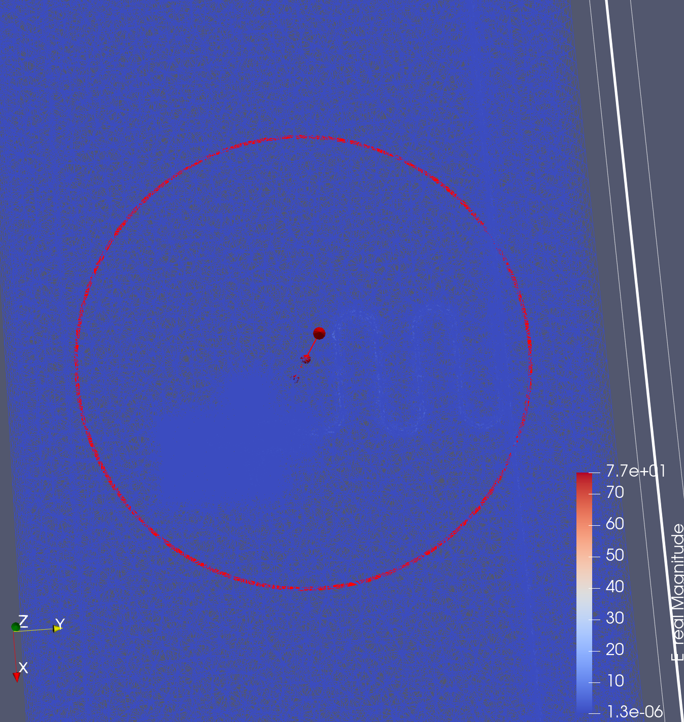
Error in plotting: 'Data array (E_real) not present in this dataset.'
Reading the eigenmode data now
[35]:
def read_csv_to_dataframe(file_path):
    return pd.read_csv(file_path)

eigen_df = read_csv_to_dataframe(os.path.join(eigen_sim._output_data_dir, 'eig.csv'))
eigen_df.columns = eigen_df.columns.str.strip()
eigen_df["kappa (kHz)"] = eigen_df["Re{f} (GHz)"] / eigen_df["Q"] * 1e6
eigen_df
[35]:
| m | Re{f} (GHz) | Im{f} (GHz) | Q | Error (Bkwd.) | Error (Abs.) | kappa (kHz) | |
|---|---|---|---|---|---|---|---|
| 0 | 1.0 | 3.136773 | 0.000142 | 11052.078980 | 7.453931e-09 | 0.001332 | 283.817505 |
| 1 | 2.0 | 7.182393 | 0.053806 | 66.745601 | 1.006761e-06 | 0.179951 | 107608.479305 |
| 2 | 3.0 | 7.984742 | 0.060560 | 65.926071 | 1.045471e-06 | 0.186871 | 121116.613403 |
| 3 | 4.0 | 9.637756 | 0.048534 | 99.290551 | 1.024503e-06 | 0.183126 | 97066.198247 |
| 4 | 5.0 | 9.940094 | 0.079461 | 62.548816 | 1.765758e-06 | 0.315623 | 158917.379265 |
| 5 | 6.0 | 10.696625 | 0.247229 | 21.638840 | 8.803714e-07 | 0.157364 | 494325.272753 |
From our requirements, we wanted a qubit frequency of 3.7 GHz and a cavity frequency of
[36]:
target_params["cavity_frequency_GHz"]
[36]:
6.98
From the simulations, it seems like mode 1 is the qubit mode (found to be 3.136 GHz) and mode 2 is the cavity mode (found to be 7.183 GHz) given their frequencies
Lets’ visualize all the eigenmodes in paraview to see if thats the case. Here are some screenshots from this toy example.
|
|
|
Mode 1: Qubit Mode | Mode 2: Cavity Mode? | Mode 3: Cavity Mode? |
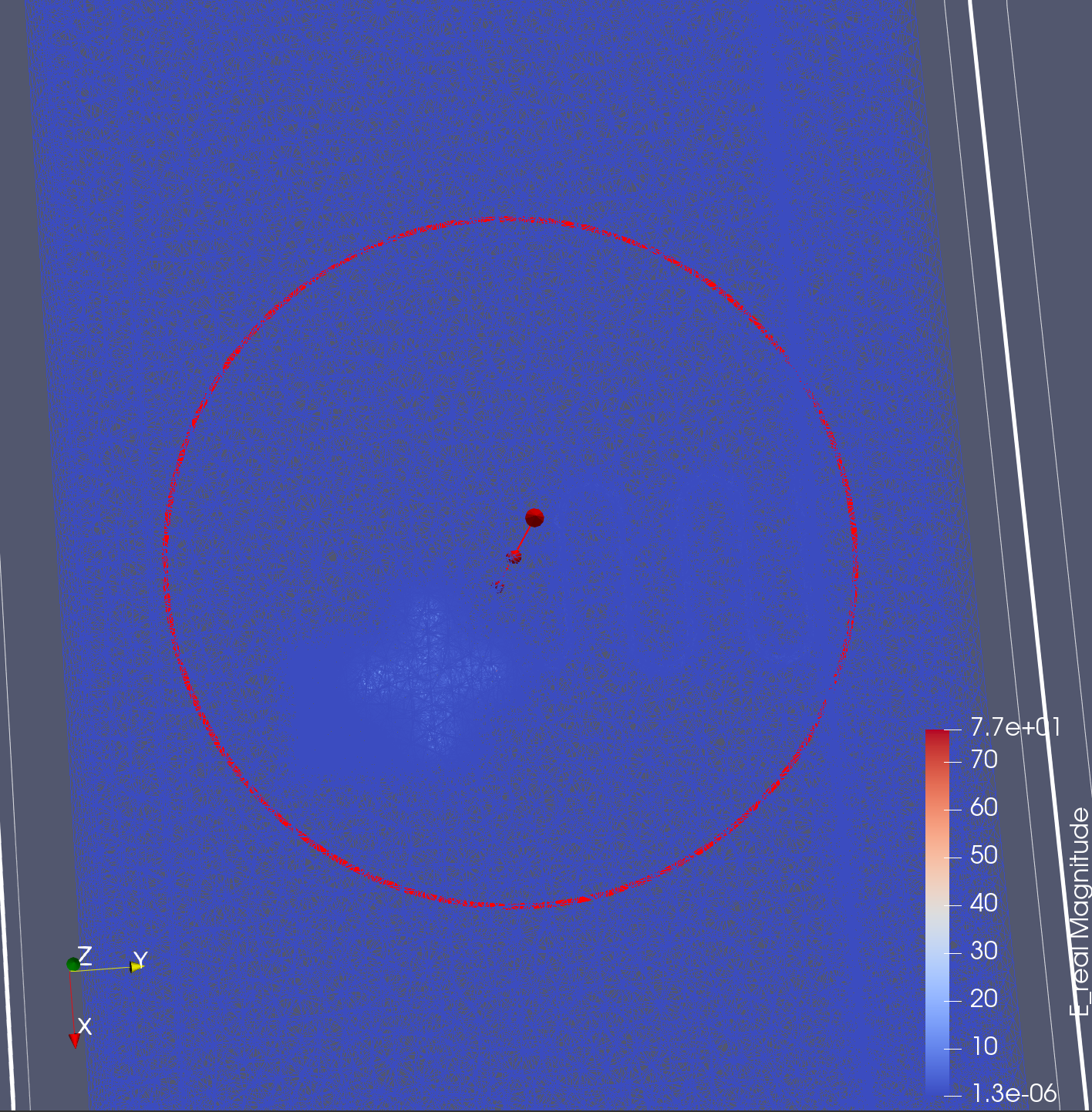
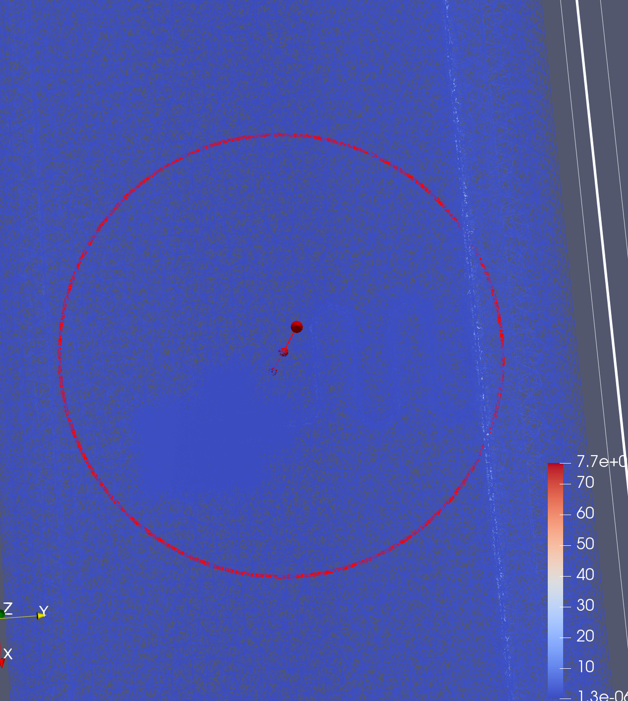
It seems like that indeed mode 1 is the qubit mode and mode 3 looks to be like the cavity mode (apologies for the bad quality of the images).
Of course, this simulation was done with really coarse hyperparameters (ran in 1.5 minutes on my 2021 Macbook Pro) so this results are somewhat promising!
EPR Calculations#
Since palace does automatic postprocessing of energy-participation ratios (EPRs) for circuit quantization and interface or bulk participation ratios for predicting dielectric loss, we can use this to do some quantum analysis from the eigenmode simulation when lumped inductive elements (i.e. josephson junctions) exist in the simulated geometry.
First, we need to retrieve the mode-port EPRs from the eigenmode simulation.
[37]:
mode_dict = eigen_sim.retrieve_mode_port_EPR_from_file(eigen_sim._output_data_dir)

#get particpation ratios and frequencies from the simulation
participation_ratios = mode_dict['mat_mode_port']
frequencies = mode_dict['eigenfrequencies']
We have identified the qubit and cavity modes from the eigenmode simulation as mode 3 and mode 4 respectively.
[38]:
qubit_idx = 0
cavity_idx = 2
[39]:
linear_qubit_freq = eigen_df['Re{f} (GHz)'][qubit_idx]*1e9
linear_res_freq = eigen_df['Re{f} (GHz)'][cavity_idx]*1e9
P_qubit = abs(participation_ratios[qubit_idx, 0])
P_cav = abs(participation_ratios[cavity_idx, 0])
[40]:
P_qubit, P_cav
[40]:
(0.9902988796, 5.021029524e-05)
Now, let’s calculate the qubit and cavity Hamiltonian parameters using these participation ratios.
[41]:
#Constants used for calculations
from scipy.constants import Planck, e, hbar

phi0 = hbar/(2*e)

#Josephson Energy (Ej) and linear inductance (Lj)
delta_super = (1.8e-4 / 2) * e
Lj = LJs[0]*1e-9
Ej = phi0**2 / Lj

#Normalize Participation Ratios
P_qubit_normalised = P_qubit / (P_qubit + P_cav)
P_cav_normalised = P_cav / (P_qubit + P_cav)

#Enter in Frequencies from Simulation
omega_qubit = 2 * np.pi * linear_qubit_freq
omega_res = 2 * np.pi * linear_res_freq

#phi zero-point fluctuations for qubit
phi_zpf_sq = P_qubit * hbar * 2 * omega_qubit  / (2*Ej)

#anharmonicity qubit (self kerr)
anharm_qubit = P_qubit**2 * hbar * omega_qubit**2 / (8*Ej)

#anharmonicity resonator (self kerr)
anharm_res = P_cav**2 * hbar * omega_res**2 / (8*Ej)

#Charging Energy (Ec)
Ec = anharm_qubit * hbar

#Total Capacitance
C_total = e**2 / (2*Ec)

#cross kerr - dispersive shit (chi)
cross_kerr = (P_qubit * P_cav * hbar * omega_qubit * omega_res) / (4*Ej)

#lamb-shift of qubit frequency
lamb_shift_qubit = anharm_qubit - cross_kerr/2

#lamb-shift of res frequency
lamb_shift_res = anharm_res - cross_kerr/2

#detuning, delta
delta = ((linear_res_freq - anharm_res/(2*np.pi)) - (linear_qubit_freq - anharm_qubit/(2*np.pi)))

#resonator-qubit coupling strength (g)
disp_shift_qubit = cross_kerr
g_rwa = np.sqrt(disp_shift_qubit * delta  * (1 + delta/anharm_qubit))

# coupling strength (g) from SQuADDS Paper
Delta = omega_res - omega_qubit      # rad/s
Sigma = omega_res + omega_qubit      # rad/s
alpha = -anharm_qubit                # rad/s (already angular)
chi = -disp_shift_qubit              # rad/s (already angular)
# Denominator (s/rad)
denom = (alpha / (Delta * (Delta - alpha))) - (alpha / (Sigma * (Sigma + alpha)))

# Convert to linear frequency in MHz (optional, for reporting)
g_rad = np.sqrt(chi / (2 * denom))     # rad/s
g_MHz = g_rad / (2 * np.pi * 1e6)    # MHz
Interesting to check what scqubits says about the Hamiltonian parameters computed using the simulation results.
[42]:
import scqubits as scq
from scqubits.core.transmon import Transmon

scq.set_units("GHz")

# Using scqubits to find the Josephson energy and charging energy using the qubit frequency and anharmonicity from EPR
qubit_freq_GHz = linear_qubit_freq/1e9 - lamb_shift_qubit/(2*np.pi*1e9)
qubit_anharm_GHz = (alpha*1e-9)/(2*np.pi)
EJ_scq, EC_scq = Transmon.find_EJ_EC(qubit_freq_GHz, qubit_anharm_GHz)


# Using scqubits to find the qubit frequency and anharmonicity now using the Josephson energy and charging energy from EP
EJ_GHz = Ej / (hbar * 2 * np.pi *  1e9)
EC_GHz = anharm_qubit  / (2*np.pi*1e9)
transmon = Transmon(EJ=EJ_GHz, EC=EC_GHz, ng=0, ncut=30)
qubit_freq_scq= transmon.E01()
anharm_qubit_scq = transmon.anharmonicity() * 1E3  # MHz

# Using scqubits to find the C_qubit capacitance

def C_qubit_from_Ec(Ec):
    """
    Calculate the capacitance (C_qubit) in fF from the charging energy (Ec) in GHz.
    """
    Ec_Joules = Ec * 1e9 * Planck
    Cs_SI = (e ** 2) / (2 * Ec_Joules)
    Cs_fF = Cs_SI * 1e15
    return Cs_fF

C_qubit_scq = C_qubit_from_Ec(EC_scq)
[43]:
hamiltonian_params = [
    ("Ej", Ej / (hbar * 2 * np.pi *  1e9), "GHz"),
    ("Ej (scqubits)", EJ_scq, "GHz"),
    ("Ec", anharm_qubit  / (2*np.pi*1e9), "GHz"),
    ("Ec (scqubits)", EC_scq, "GHz"),
    ("Ej/Ec", Ej/Ec, "unitless"),
    ("Ej/Ec (scqubits)", EJ_scq/EC_scq, "unitless"),
    ("Lj", Lj/1e-9, "nH"),
    ("C_qubit", C_total/1e-15, "fF"),
    ("C_qubit (scqubits)", C_qubit_scq, "fF"),
    ("C_qubit (from SQuADDS DB)", results["cross_to_claw"].values[0]+results["cross_to_ground"].values[0], "fF"),
    ("Participation Ratio Qubit", P_qubit, "unitless"),
    ("Participation Ratio Qubit (Normalized)", P_qubit_normalised, "unitless"),
    ("Participation Ratio Cavity", P_cav, "unitless"),
    ("Participation Ratio Cavity (Normalized)", P_cav_normalised, "unitless"),
    ("Linear Qubit Frequency", linear_qubit_freq/1e9, "GHz"),
    ("Qubit Frequency", linear_qubit_freq/1e9 - lamb_shift_qubit/(2*np.pi*1e9), "GHz"),
    ("Qubit Frequency (scqubits)", qubit_freq_scq, "GHz"),
    ("Qubit Frequency (from SQuADDS DB)", results["qubit_frequency_GHz"].values[0], "GHz"),
    ("Qubit Anharmonicity", anharm_qubit / (2*np.pi*1e6), "MHz"),
    ("Qubit Anharmonicity (scqubits)", -anharm_qubit_scq, "MHz"),
    ("Qubit Anharmonicity (from SQuADDS DB)", - results["anharmonicity_MHz"].values[0], "MHz"),
    ("Linear Cavity Frequency", linear_res_freq/1e9, "GHz"),
    ("Cavity Frequency", linear_res_freq/1e9 - lamb_shift_res/(2*np.pi*1e9), "GHz"),
    ("Cavity Anharmonicity", anharm_res / (2*np.pi*1e6), "MHz"),
    ("Dispersive Shift (chi)", cross_kerr/ (2*np.pi*1e6), "MHz"),
    ("Cavity-Qubit Coupling [Ref. SQuADDS], g", g_MHz, "MHz"),
    ("Cavity-Qubit Coupling [RWA], g", g_rwa/(2*np.pi*1e6), "MHz"),
    ("Detuning", delta/1e9, "GHz"),
    ("Flux_ZPF_squared", phi_zpf_sq, "unitless"),
]

# Create DataFrame
hamiltonian_df = pd.DataFrame(hamiltonian_params, columns=["Parameter", "Value", "Unit"])

# Function to format values
def format_float_six_decimal(val, idx):
    return f"{val:.6f}"

# Apply formatting
hamiltonian_df['Value'] = [
    format_float_six_decimal(val, idx) for idx, val in enumerate(hamiltonian_df['Value'])
]

print(hamiltonian_df.to_string(index=False))
                              Parameter      Value     Unit
                                     Ej  10.278024      GHz
                          Ej (scqubits)  11.401425      GHz
                                     Ec   0.117354      GHz
                          Ec (scqubits)   0.107476      GHz
                                  Ej/Ec  87.581095 unitless
                       Ej/Ec (scqubits) 106.083580 unitless
                                     Lj  15.903982       nH
                                C_qubit 165.057588       fF
                     C_qubit (scqubits) 180.228631       fF
              C_qubit (from SQuADDS DB) 107.321280       fF
              Participation Ratio Qubit   0.990299 unitless
 Participation Ratio Qubit (Normalized)   0.999949 unitless
             Participation Ratio Cavity   0.000050 unitless
Participation Ratio Cavity (Normalized)   0.000051 unitless
                 Linear Qubit Frequency   3.136773      GHz
                        Qubit Frequency   3.019434      GHz
             Qubit Frequency (scqubits)   2.984043      GHz
      Qubit Frequency (from SQuADDS DB)   3.662130      GHz
                    Qubit Anharmonicity 117.354370      MHz
         Qubit Anharmonicity (scqubits) 129.507341      MHz
  Qubit Anharmonicity (from SQuADDS DB) 205.109839      MHz
                Linear Cavity Frequency   7.984742      GHz
                       Cavity Frequency   7.984758      GHz
                   Cavity Anharmonicity   0.000002      MHz
                 Dispersive Shift (chi)   0.030292      MHz
Cavity-Qubit Coupling [Ref. SQuADDS], g  62.189165      MHz
         Cavity-Qubit Coupling [RWA], g  13.606631      MHz
                               Detuning   4.965323      GHz
                       Flux_ZPF_squared   0.302232 unitless
Drivenmodal Simulations#
Now, we show how to run Drivenmodal simulations to get the scattering parameters. Let’s use the same qubit-cavity geometry as the eigenmodal simulation for this.
[45]:
from SQDMetal.PALACE.Frequency_Driven_Simulation import PALACE_Driven_Simulation

#Eigenmode Simulation Options
user_defined_options = {
                 "mesh_refinement":  0,                             #refines mesh in PALACE - essetially divides every mesh element in half
                 "dielectric_material": "silicon",                  #choose dielectric material - 'silicon' or 'sapphire'
                 "solns_to_save": 4,                                #number of electromagnetic field visualizations to save
                 "solver_order": 1,                                 #increasing solver order increases accuracy of simulation, but significantly increases sim time
                 "solver_tol": 1.0e-3,                              #error residual tolerance foriterative solver
                 "solver_maxits": 3,                              #number of solver iterations
                 "mesh_max": 120e-3,                                #maxiumum element size for the mesh in mm
                 "mesh_min": 10e-3,                                 #minimum element size for the mesh in mm
                 "mesh_sampling": 130,                              #number of points to mesh along a geometry
                 "fillet_resolution":12,
                 "num_cpus": 10,                                      #number of CPU cores to use for simulation
                 "palace_dir":path_to_palace
                }

#Create the Palace Frequency Driven simulation
driven_sim = PALACE_Driven_Simulation(
    name='qubit-cavity-driven',                  #name of simulation
    metal_design=design,                              #feed in qiskit metal design
    sim_parent_directory="sims/",                     #choose directory where mesh file, config file and HPC batch file will be saved
    mode='simPC',                                     #choose simulation mode 'HPC' or 'simPC'
    meshing='GMSH',                                   #choose meshing 'GMSH' or 'COMSOL'
    user_options=user_defined_options,                #provide options chosen above
    view_design_gmsh_gui=False,                       #view design in GMSH gui
    create_files=True                                 #create mesh, config and HPC batch files
)
[46]:
from SQDMetal.Utilities.Materials import MaterialInterface

# Add metallic elements and ground plane
driven_sim.add_metallic(1, threshold=1e-10, fuse_threshold=1e-10)
driven_sim.add_ground_plane(threshold=1e-10)

# Fine-mesh the transmon cross qubit region
driven_sim.fine_mesh_in_rectangle(0.2875e-3, -1.2e-3, 0.63e-3, -1.72e-3, min_size=15e-6, max_size=120e-6)

# Add in the RF ports
driven_sim.create_port_CPW_on_Launcher('LP1', 20e-6)
driven_sim.create_port_CPW_on_Launcher('LP2', 20e-6)
driven_sim.create_port_JosephsonJunction('junction', L_J=LJs[0]*1e-9, C_J=10e-15)  # Guessing the C_J value

# Fine-mesh routed paths
driven_sim.fine_mesh_around_comp_boundaries(['feedline', 'resonator'], min_size=25e-6, max_size=250e-6)
driven_sim.fine_mesh_around_comp_boundaries(['xmon'], min_size=14e-6, max_size=75e-6)

# Setup EPR interfaces
driven_sim.setup_EPR_interfaces(
    metal_air=MaterialInterface('Aluminium-Vacuum'),
    substrate_air=MaterialInterface('Silicon-Vacuum'),
    substrate_metal=MaterialInterface('Silicon-Aluminium')
)
[47]:
# Set frequency sweep parameters (in GHz)
driven_sim.set_freq_values(
    startGHz=3,    # starting frequency in GHz
    endGHz=10,     # end frequency in GHz
    stepGHz=0.5    # frequency step size in GHz
)
[48]:
# Prepare and run simulation
driven_sim.prepare_simulation()
Directory 'qubit-cavity-driven' created
NOTE: If you are using a palace build that is from 2025, you will need to remove the Excitation key from the LumpedPort boundary condition in the sim_config.json file so please execute the following cell.
If you are using a palace build that is from 2024 or older, you should skip this cell.
[ ]:
import json

with open(driven_sim._sim_config) as file:
    sim_config_dict = json.load(file)

del sim_config_dict["Boundaries"]["LumpedPort"][0]["Excitation"]

with open(eigen_sim._sim_config, 'w') as file:
    json.dump(sim_config_dict, file, indent=4)
[49]:
results = driven_sim.run()
>> /opt/homebrew/bin/mpirun -n 10 /Users/shanto/LFL/palace/build/bin/palace-arm64.bin qubit-cavity-driven.json

_____________     _______
_____   __   \____ __   /____ ____________
____   /_/  /  __ ` /  /  __ ` /  ___/  _ \
___   _____/  /_/  /  /  /_/  /  /__/  ___/
  /__/     \___,__/__/\___,__/\_____\_____/

Git changeset ID: v0.13.0-117-g748660c
Running with 10 MPI processes
Device configuration: cpu
Memory configuration: host-std
libCEED backend: /cpu/self/xsmm/blocked

Added 2574 elements in 2 iterations of local bisection for under-resolved interior boundaries
Added 5333 duplicate vertices for interior boundaries in the mesh
Added 12701 duplicate boundary elements for interior boundaries in the mesh
Added 1550 boundary elements for material interfaces to the mesh
Finished partitioning mesh into 10 subdomains

Characteristic length and time scales:
 L₀ = 5.520e-03 m, t₀ = 1.841e-02 ns

Mesh curvature order: 1
Mesh bounding box:
 (Xmin, Ymin, Zmin) = (-2.760e-03, -2.440e-03, -2.800e-04) m
 (Xmax, Ymax, Zmax) = (+2.760e-03, +4.400e-04, +2.800e-04) m

Parallel Mesh Stats:

                minimum     average     maximum       total
 vertices          2786        3522        3859       35223
 edges            18749       20919       22124      209195
 faces            31110       32653       33699      326538
 elements         15011       15256       15457      152568
 neighbors            2           4           5

            minimum     maximum
 h      0.000513927   0.0271869
 kappa      1.01967     157.435

Configuring Robin absorbing BC (order 1) at attributes:
 13

Configuring Robin impedance BC for lumped ports at attributes:
 5: Rs = 6.667e+01 Ω/sq, n = (+0.0, +0.0, +1.0)
 6: Rs = 6.667e+01 Ω/sq, n = (+0.0, +0.0, -1.0)
 7: Rs = 6.667e+01 Ω/sq, n = (-0.0, +0.0, +1.0)
 8: Rs = 6.667e+01 Ω/sq, n = (+0.0, +0.0, -1.0)
 9: Ls = 5.725e-09 H/sq, Cs = 2.778e-14 F/sq, n = (+0.0, +0.0, +1.0)

Configuring lumped port circuit properties:
 Index = 1: R = 5.000e+01 Ω
 Index = 2: R = 5.000e+01 Ω
 Index = 3: L = 1.590e-08 H, C = 1.000e-14 F

Configuring lumped port excitation source term at attributes:
 5: Index = 1
 6: Index = 1

Configuring Dirichlet PEC BC at attributes:
 1-4

Computing frequency response for:
 Lumped port excitation specified on ports 1

Assembling system matrices, number of global unknowns:
 H1 (p = 1): 35223, ND (p = 1): 209195, RT (p = 1): 326538
 Operator assembly level: Partial
 Mesh geometries:
  Tetrahedron: P = 6, Q = 4 (quadrature order = 2)

Assembling multigrid hierarchy:
 Level 0 (p = 1): 209195 unknowns, 3111237 NNZ
 Level 0 (auxiliary) (p = 1): 35223 unknowns, 467972 NNZ

It 1/15: ω/2π = 3.000e+00 GHz (elapsed time = 2.91e-07 s)

Residual norms for FGMRES solve
0 (restart 0) KSP residual norm 6.351240e-01
1 (restart 0) KSP residual norm 3.601434e-01
2 (restart 0) KSP residual norm 3.457708e-02
3 (restart 1) KSP residual norm 5.712683e-03
FGMRES solver did NOT converge in 3 iterations (avg. reduction factor: 2.080e-01)

--> Warning!
Linear solver did not converge, norm(Ax-b)/norm(b) = 8.995e-03 (norm(b) = 6.351e-01)!

 Sol. ||E|| = 1.080985e+01 (||RHS|| = 6.351240e-01)
 Field energy E (2.658e-02 J) + H (8.606e-03 J) = 3.519e-02 J
 Updating solution error estimates
 S[1][1] = -6.783e-01-3.388e-01i, |S[1][1]| = -2.404e+00, arg(S[1][1]) = -1.535e+02
 S[2][1] = +2.911e-01-5.831e-01i, |S[2][1]| = -3.719e+00, arg(S[2][1]) = -6.347e+01
 S[3][1] = +0.000e+00+0.000e+00i, |S[3][1]| = -inf, arg(S[3][1]) = +0.000e+00

 Wrote fields to disk at step 1

It 2/15: ω/2π = 3.500e+00 GHz (elapsed time = 1.14e+01 s)

Residual norms for FGMRES solve
0 (restart 0) KSP residual norm 9.903109e-02
1 (restart 0) KSP residual norm 8.059919e-02
2 (restart 0) KSP residual norm 1.326503e-02
3 (restart 1) KSP residual norm 5.781395e-03
FGMRES solver did NOT converge in 3 iterations (avg. reduction factor: 1.983e-01)

--> Warning!
Linear solver did not converge, norm(Ax-b)/norm(b) = 7.802e-03 (norm(b) = 7.410e-01)!

 Sol. ||E|| = 9.294195e+00 (||RHS|| = 7.409780e-01)
 Field energy E (1.967e-02 J) + H (8.991e-03 J) = 2.866e-02 J
 Updating solution error estimates
 S[1][1] = -7.525e-01-2.548e-01i, |S[1][1]| = -1.998e+00, arg(S[1][1]) = -1.613e+02
 S[2][1] = +2.044e-01-5.429e-01i, |S[2][1]| = -4.729e+00, arg(S[2][1]) = -6.937e+01
 S[3][1] = +0.000e+00+0.000e+00i, |S[3][1]| = -inf, arg(S[3][1]) = +0.000e+00

It 3/15: ω/2π = 4.000e+00 GHz (elapsed time = 1.69e+01 s)

Residual norms for FGMRES solve
0 (restart 0) KSP residual norm 1.008076e-01
1 (restart 0) KSP residual norm 7.244153e-02
2 (restart 0) KSP residual norm 2.058542e-02
3 (restart 1) KSP residual norm 6.419817e-03
FGMRES solver did NOT converge in 3 iterations (avg. reduction factor: 1.964e-01)

--> Warning!
Linear solver did not converge, norm(Ax-b)/norm(b) = 7.581e-03 (norm(b) = 8.468e-01)!

 Sol. ||E|| = 8.579163e+00 (||RHS|| = 8.468320e-01)
 Field energy E (1.679e-02 J) + H (9.388e-03 J) = 2.618e-02 J
 Updating solution error estimates
 S[1][1] = -7.918e-01-1.988e-01i, |S[1][1]| = -1.762e+00, arg(S[1][1]) = -1.659e+02
 S[2][1] = +1.500e-01-5.324e-01i, |S[2][1]| = -5.144e+00, arg(S[2][1]) = -7.427e+01
 S[3][1] = +0.000e+00+0.000e+00i, |S[3][1]| = -inf, arg(S[3][1]) = +0.000e+00

It 4/15: ω/2π = 4.500e+00 GHz (elapsed time = 2.42e+01 s)

Residual norms for FGMRES solve
0 (restart 0) KSP residual norm 1.021443e-01
1 (restart 0) KSP residual norm 6.477930e-02
2 (restart 0) KSP residual norm 2.157044e-02
3 (restart 1) KSP residual norm 1.044909e-02
FGMRES solver did NOT converge in 3 iterations (avg. reduction factor: 2.222e-01)

--> Warning!
Linear solver did not converge, norm(Ax-b)/norm(b) = 1.097e-02 (norm(b) = 9.527e-01)!

 Sol. ||E|| = 7.907910e+00 (||RHS|| = 9.526860e-01)
 Field energy E (1.428e-02 J) + H (9.791e-03 J) = 2.407e-02 J
 Updating solution error estimates
 S[1][1] = -8.197e-01-1.373e-01i, |S[1][1]| = -1.606e+00, arg(S[1][1]) = -1.705e+02
 S[2][1] = +1.034e-01-5.178e-01i, |S[2][1]| = -5.547e+00, arg(S[2][1]) = -7.870e+01
 S[3][1] = +0.000e+00+0.000e+00i, |S[3][1]| = -inf, arg(S[3][1]) = +0.000e+00

It 5/15: ω/2π = 5.000e+00 GHz (elapsed time = 3.04e+01 s)

Residual norms for FGMRES solve
0 (restart 0) KSP residual norm 1.039076e-01
1 (restart 0) KSP residual norm 6.272732e-02
2 (restart 0) KSP residual norm 5.587032e-02
3 (restart 1) KSP residual norm 2.058066e-02
FGMRES solver did NOT converge in 3 iterations (avg. reduction factor: 2.689e-01)

--> Warning!
Linear solver did not converge, norm(Ax-b)/norm(b) = 1.944e-02 (norm(b) = 1.059e+00)!

 Sol. ||E|| = 7.378380e+00 (||RHS|| = 1.058540e+00)
 Field energy E (1.245e-02 J) + H (1.018e-02 J) = 2.263e-02 J
 Updating solution error estimates
 S[1][1] = -8.356e-01-7.813e-02i, |S[1][1]| = -1.523e+00, arg(S[1][1]) = -1.747e+02
 S[2][1] = +6.471e-02-5.062e-01i, |S[2][1]| = -5.842e+00, arg(S[2][1]) = -8.272e+01
 S[3][1] = +0.000e+00+0.000e+00i, |S[3][1]| = -inf, arg(S[3][1]) = +0.000e+00

 Wrote fields to disk at step 5

It 6/15: ω/2π = 5.500e+00 GHz (elapsed time = 3.83e+01 s)

Residual norms for FGMRES solve
0 (restart 0) KSP residual norm 1.085018e-01
1 (restart 0) KSP residual norm 6.991534e-02
2 (restart 0) KSP residual norm 6.988851e-02
3 (restart 1) KSP residual norm 5.191527e-02
FGMRES solver did NOT converge in 3 iterations (avg. reduction factor: 3.546e-01)

--> Warning!
Linear solver did not converge, norm(Ax-b)/norm(b) = 4.459e-02 (norm(b) = 1.164e+00)!

 Sol. ||E|| = 6.921427e+00 (||RHS|| = 1.164394e+00)
 Field energy E (1.097e-02 J) + H (1.020e-02 J) = 2.117e-02 J
 Updating solution error estimates
 S[1][1] = -8.341e-01-2.251e-02i, |S[1][1]| = -1.573e+00, arg(S[1][1]) = -1.785e+02
 S[2][1] = +3.688e-02-4.904e-01i, |S[2][1]| = -6.164e+00, arg(S[2][1]) = -8.570e+01
 S[3][1] = +0.000e+00+0.000e+00i, |S[3][1]| = -inf, arg(S[3][1]) = +0.000e+00

It 7/15: ω/2π = 6.000e+00 GHz (elapsed time = 4.60e+01 s)

Residual norms for FGMRES solve
0 (restart 0) KSP residual norm 1.347054e-01
1 (restart 0) KSP residual norm 1.238462e-01
2 (restart 0) KSP residual norm 1.106825e-01
3 (restart 1) KSP residual norm 1.097831e-01
FGMRES solver did NOT converge in 3 iterations (avg. reduction factor: 4.421e-01)

--> Warning!
Linear solver did not converge, norm(Ax-b)/norm(b) = 8.643e-02 (norm(b) = 1.270e+00)!

 Sol. ||E|| = 6.235652e+00 (||RHS|| = 1.270248e+00)
 Field energy E (8.901e-03 J) + H (9.715e-03 J) = 1.862e-02 J
 Updating solution error estimates
 S[1][1] = -8.310e-01+3.706e-02i, |S[1][1]| = -1.599e+00, arg(S[1][1]) = +1.774e+02
 S[2][1] = +7.673e-03-4.604e-01i, |S[2][1]| = -6.737e+00, arg(S[2][1]) = -8.905e+01
 S[3][1] = +0.000e+00+0.000e+00i, |S[3][1]| = -inf, arg(S[3][1]) = +0.000e+00

It 8/15: ω/2π = 6.500e+00 GHz (elapsed time = 5.18e+01 s)

Residual norms for FGMRES solve
0 (restart 0) KSP residual norm 2.011330e-01
1 (restart 0) KSP residual norm 1.985118e-01
2 (restart 0) KSP residual norm 1.821145e-01
3 (restart 1) KSP residual norm 1.661144e-01
FGMRES solver did NOT converge in 3 iterations (avg. reduction factor: 4.942e-01)

--> Warning!
Linear solver did not converge, norm(Ax-b)/norm(b) = 1.207e-01 (norm(b) = 1.376e+00)!

 Sol. ||E|| = 6.030714e+00 (||RHS|| = 1.376102e+00)
 Field energy E (8.322e-03 J) + H (1.012e-02 J) = 1.845e-02 J
 Updating solution error estimates
 S[1][1] = -8.530e-01+8.478e-02i, |S[1][1]| = -1.339e+00, arg(S[1][1]) = +1.743e+02
 S[2][1] = -3.345e-02-4.634e-01i, |S[2][1]| = -6.659e+00, arg(S[2][1]) = -9.413e+01
 S[3][1] = +0.000e+00+0.000e+00i, |S[3][1]| = -inf, arg(S[3][1]) = +0.000e+00

It 9/15: ω/2π = 7.000e+00 GHz (elapsed time = 5.75e+01 s)

Residual norms for FGMRES solve
0 (restart 0) KSP residual norm 2.526932e-01
1 (restart 0) KSP residual norm 2.514240e-01
2 (restart 0) KSP residual norm 2.352636e-01
3 (restart 1) KSP residual norm 1.872347e-01
FGMRES solver did NOT converge in 3 iterations (avg. reduction factor: 5.018e-01)

--> Warning!
Linear solver did not converge, norm(Ax-b)/norm(b) = 1.263e-01 (norm(b) = 1.482e+00)!

 Sol. ||E|| = 6.063368e+00 (||RHS|| = 1.481956e+00)
 Field energy E (8.431e-03 J) + H (1.064e-02 J) = 1.907e-02 J
 Updating solution error estimates
 S[1][1] = -8.490e-01+1.257e-01i, |S[1][1]| = -1.328e+00, arg(S[1][1]) = +1.716e+02
 S[2][1] = -6.245e-02-4.702e-01i, |S[2][1]| = -6.478e+00, arg(S[2][1]) = -9.756e+01
 S[3][1] = +0.000e+00+0.000e+00i, |S[3][1]| = -inf, arg(S[3][1]) = +0.000e+00

 Wrote fields to disk at step 9

It 10/15: ω/2π = 7.500e+00 GHz (elapsed time = 6.41e+01 s)

Residual norms for FGMRES solve
0 (restart 0) KSP residual norm 2.703739e-01
1 (restart 0) KSP residual norm 2.442628e-01
2 (restart 0) KSP residual norm 2.237861e-01
3 (restart 1) KSP residual norm 1.848211e-01
FGMRES solver did NOT converge in 3 iterations (avg. reduction factor: 4.883e-01)

--> Warning!
Linear solver did not converge, norm(Ax-b)/norm(b) = 1.164e-01 (norm(b) = 1.588e+00)!

 Sol. ||E|| = 6.104483e+00 (||RHS|| = 1.587810e+00)
 Field energy E (8.570e-03 J) + H (1.135e-02 J) = 1.992e-02 J
 Updating solution error estimates
 S[1][1] = -8.184e-01+1.706e-01i, |S[1][1]| = -1.556e+00, arg(S[1][1]) = +1.682e+02
 S[2][1] = -9.212e-02-4.720e-01i, |S[2][1]| = -6.359e+00, arg(S[2][1]) = -1.010e+02
 S[3][1] = +0.000e+00+0.000e+00i, |S[3][1]| = -inf, arg(S[3][1]) = +0.000e+00

It 11/15: ω/2π = 8.000e+00 GHz (elapsed time = 6.98e+01 s)

Residual norms for FGMRES solve
0 (restart 0) KSP residual norm 2.648449e-01
1 (restart 0) KSP residual norm 2.529848e-01
2 (restart 0) KSP residual norm 2.470227e-01
3 (restart 1) KSP residual norm 2.132539e-01
FGMRES solver did NOT converge in 3 iterations (avg. reduction factor: 5.012e-01)

--> Warning!
Linear solver did not converge, norm(Ax-b)/norm(b) = 1.259e-01 (norm(b) = 1.694e+00)!

 Sol. ||E|| = 6.074015e+00 (||RHS|| = 1.693664e+00)
 Field energy E (8.485e-03 J) + H (1.086e-02 J) = 1.934e-02 J
 Updating solution error estimates
 S[1][1] = -7.818e-01+1.886e-01i, |S[1][1]| = -1.892e+00, arg(S[1][1]) = +1.664e+02
 S[2][1] = -1.115e-01-4.599e-01i, |S[2][1]| = -6.498e+00, arg(S[2][1]) = -1.036e+02
 S[3][1] = +0.000e+00+0.000e+00i, |S[3][1]| = -inf, arg(S[3][1]) = +0.000e+00

It 12/15: ω/2π = 8.500e+00 GHz (elapsed time = 7.59e+01 s)

Residual norms for FGMRES solve
0 (restart 0) KSP residual norm 2.984142e-01
1 (restart 0) KSP residual norm 2.575522e-01
2 (restart 0) KSP residual norm 2.376679e-01
3 (restart 1) KSP residual norm 2.322283e-01
FGMRES solver did NOT converge in 3 iterations (avg. reduction factor: 5.053e-01)

--> Warning!
Linear solver did not converge, norm(Ax-b)/norm(b) = 1.291e-01 (norm(b) = 1.800e+00)!

 Sol. ||E|| = 6.126870e+00 (||RHS|| = 1.799518e+00)
 Field energy E (8.574e-03 J) + H (1.221e-02 J) = 2.078e-02 J
 Updating solution error estimates
 S[1][1] = -7.212e-01+2.521e-01i, |S[1][1]| = -2.338e+00, arg(S[1][1]) = +1.607e+02
 S[2][1] = -1.542e-01-4.445e-01i, |S[2][1]| = -6.550e+00, arg(S[2][1]) = -1.091e+02
 S[3][1] = +0.000e+00+0.000e+00i, |S[3][1]| = -inf, arg(S[3][1]) = +0.000e+00

It 13/15: ω/2π = 9.000e+00 GHz (elapsed time = 8.20e+01 s)

Residual norms for FGMRES solve
0 (restart 0) KSP residual norm 3.080933e-01
1 (restart 0) KSP residual norm 3.057754e-01
2 (restart 0) KSP residual norm 2.924240e-01
3 (restart 1) KSP residual norm 2.864515e-01
FGMRES solver did NOT converge in 3 iterations (avg. reduction factor: 5.317e-01)

--> Warning!
Linear solver did not converge, norm(Ax-b)/norm(b) = 1.503e-01 (norm(b) = 1.905e+00)!

 Sol. ||E|| = 6.185118e+00 (||RHS|| = 1.905372e+00)
 Field energy E (8.678e-03 J) + H (1.174e-02 J) = 2.042e-02 J
 Updating solution error estimates
 S[1][1] = -7.057e-01+2.713e-01i, |S[1][1]| = -2.429e+00, arg(S[1][1]) = +1.590e+02
 S[2][1] = -1.719e-01-4.405e-01i, |S[2][1]| = -6.506e+00, arg(S[2][1]) = -1.113e+02
 S[3][1] = +0.000e+00+0.000e+00i, |S[3][1]| = -inf, arg(S[3][1]) = +0.000e+00

 Wrote fields to disk at step 13

It 14/15: ω/2π = 9.500e+00 GHz (elapsed time = 9.28e+01 s)

Residual norms for FGMRES solve
0 (restart 0) KSP residual norm 3.707691e-01
1 (restart 0) KSP residual norm 3.632131e-01
2 (restart 0) KSP residual norm 3.557204e-01
3 (restart 1) KSP residual norm 3.442652e-01
FGMRES solver did NOT converge in 3 iterations (avg. reduction factor: 5.552e-01)

--> Warning!
Linear solver did not converge, norm(Ax-b)/norm(b) = 1.712e-01 (norm(b) = 2.011e+00)!

 Sol. ||E|| = 6.305533e+00 (||RHS|| = 2.011226e+00)
 Field energy E (9.056e-03 J) + H (1.203e-02 J) = 2.109e-02 J
 Updating solution error estimates
 S[1][1] = -6.764e-01+3.036e-01i, |S[1][1]| = -2.599e+00, arg(S[1][1]) = +1.558e+02
 S[2][1] = -2.045e-01-4.389e-01i, |S[2][1]| = -6.299e+00, arg(S[2][1]) = -1.150e+02
 S[3][1] = +0.000e+00+0.000e+00i, |S[3][1]| = -inf, arg(S[3][1]) = +0.000e+00

It 15/15: ω/2π = 1.000e+01 GHz (elapsed time = 9.95e+01 s)

Residual norms for FGMRES solve
0 (restart 0) KSP residual norm 4.292106e-01
1 (restart 0) KSP residual norm 4.106243e-01
2 (restart 0) KSP residual norm 3.951131e-01
3 (restart 1) KSP residual norm 3.853653e-01
FGMRES solver did NOT converge in 3 iterations (avg. reduction factor: 5.667e-01)

--> Warning!
Linear solver did not converge, norm(Ax-b)/norm(b) = 1.820e-01 (norm(b) = 2.117e+00)!

 Sol. ||E|| = 6.533716e+00 (||RHS|| = 2.117080e+00)
 Field energy E (9.772e-03 J) + H (1.262e-02 J) = 2.240e-02 J
 Updating solution error estimates
 S[1][1] = -6.488e-01+3.379e-01i, |S[1][1]| = -2.716e+00, arg(S[1][1]) = +1.525e+02
 S[2][1] = -2.431e-01-4.430e-01i, |S[2][1]| = -5.928e+00, arg(S[2][1]) = -1.188e+02
 S[3][1] = +0.000e+00+0.000e+00i, |S[3][1]| = -inf, arg(S[3][1]) = +0.000e+00

Completed 0 iterations of adaptive mesh refinement (AMR):
 Indicator norm = 8.723e-01, global unknowns = 209195
 Max. iterations = 0, tol. = 1.000e-02

Elapsed Time Report (s)           Min.        Max.        Avg.
==============================================================
Initialization                   3.129       3.141       3.136
Operator Construction            8.549       8.879       8.721
Linear Solve                     3.889       3.961       3.926
  Setup                          2.885       3.214       3.040
  Preconditioner                43.063      43.134      43.099
Estimation                       0.528       0.618       0.578
  Construction                   2.416       2.418       2.417
  Solve                         38.133      38.194      38.168
Postprocessing                   2.555       2.632       2.584
Disk IO                          6.128       6.131       6.129
--------------------------------------------------------------
Total                          111.896     111.913     111.910
For an accurate solution, please increase meshing and reduce the tolerance.
Work In Progress ⏳#
We are studying the hyper-parameters needed to converge our simulations to that of Ansys/experimentally verified results with palace. Once that is done, we will update this tutorial with a more comprehensive guide and native API
License#
This code is a part of SQuADDS
Developed by Sadman Ahmed Shanto
This tutorial is written by Sadman Ahmed Shanto
© Copyright Sadman Ahmed Shanto & Eli Levenson-Falk 2025.
This code is licensed under the MIT License. You may obtain a copy of this license in the LICENSE.txt file in the root directory of this source tree.
Any modifications or derivative works of this code must retain thiscopyright notice, and modified files need to carry a notice indicatingthat they have been altered from the originals.